
Computing Vertex Gaussian Curvature on the GPU
Computing the Gaussian curvature for each vertex on a mesh is straightforward. We construct a halfedge data structure (HEDS) and use the lengths of each edge to find angle defect. This algorithm is ripe for parallelization while posing an interesting challenge in defining a parallel-compatible HEDS. It also serves as a great introduction to using GPUs.
This program contains two notable components: a basic implementation of a halfedge data structure (HEDS) and GPU kernel code for computing vertex Gaussian curvature. The HEDS implementation can be found under include/halfedge2.hpp and src/halfedge2.cpp. There are 3 main files: src/main.cpp (a basic linear vertex Gaussian curvature computation with a pointer-based HEDS), src/main.hip (a GPU implementation of the algorithm using AMD’s HIP), and src/main.cu (the same GPU implementation but written in CUDA). Instructions for building and running the program are listed above.
Discrete Vertex Gaussian Curvature
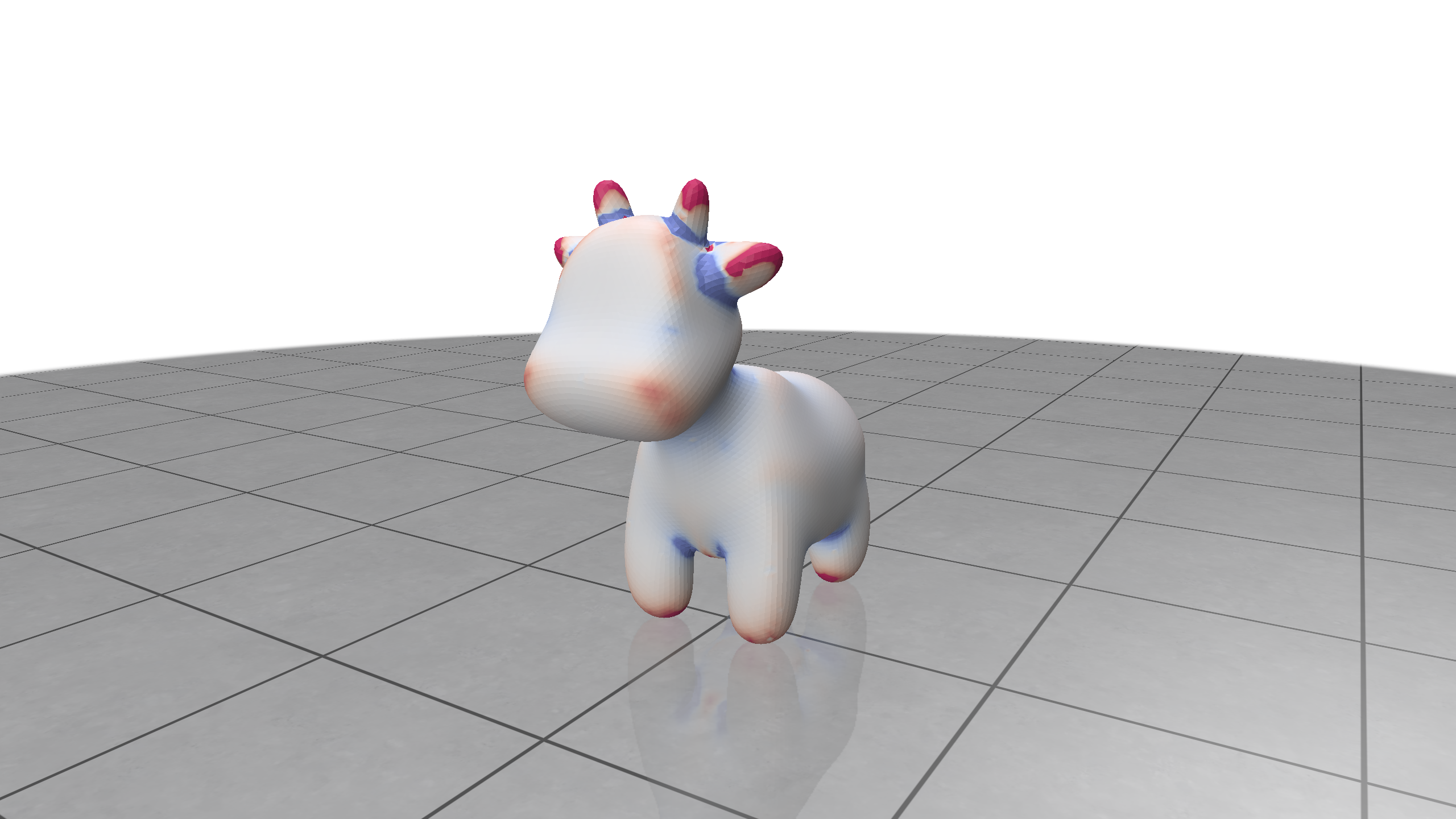
“Vertex Gaussian curvature” refers to the angle defect around a vertex $i$, which is analogous to differential Gaussian curvature on a smooth surface. On a triangular mesh, computing the the curvature on a vertex only involves the edge lengths of the faces that include $i$. Assuming edge lengths have already been computed, the angle incident to $i$ on the neighboring face $f$ ($\theta_f^i$) can be computed using the Law of Cosines: \(\theta_f^i = \arccos(\frac{a^2+b^2-c^2}{2ab}),\) where $a, b$ are the lengths of the edges containing $i$ in the face $f$, and $c$ is the length of the edge opposite to $i$.
After computing $\theta_f^i$ for each face neighboring $i$ (we denote this set of faces as $\mathcal{F}_i$), we compute the vertex Gaussian curvature at $i$ as \(K_i = 2\pi - \sum_{f \in \mathcal{F}_i} \theta_f^i.\)
The Halfedge Data Structure (HEDS)
To represent a mesh, I used a Halfedge Data Structure (HEDS). In a HEDS, a directional halfedge is used to connect vertices and denote orientation. Each vertex has a pointer to an outgoing halfedge. Halfedges themselves have pointers to the “next” halfedge, as well as their “twin.”
Given a triangular face containing vertices $i,j,k$, we can assign the halfedges $\vec{ij}, \vec{jk}, \vec{ki}$ to give a consistent orientation of the face. For the halfedge $\vec{ij}$, $\vec{ij}$.next $= \vec{jk}$ and $\vec{jk}$.next $= \vec{ki}$, so successively accessing .next on a halfedge traverses the face. $\vec{ij}$.twin $= \vec{ji}$, which connects the same two vertices but in the opposite direction.
With just these primitives, we can define an oriented mesh, as well as traverse it. In particular there are two operations we use to find $\mathcal{F}_i$. To find all outgoing edges from $i$, we track the initial $i$.outgoingHE and iteratively call .twin.next until we reach the initial edge again. Finding each face is similar — for each outgoing halfedge of $i$, the second and third edges of each face are .next and .next.next, respectively.
Pointer- vs. Index-Based HEDS
A HEDS can come in two flavors: pointer-based and index-based. In a pointer-based structure, halfedges are referenced directly by their memory address. This is pretty straightforward to implement, and allows us to leverage classes and structs in defining Vertex and HalfEdge objects. However — as we will discuss later — this implementation does not port easily to GPU memory architectures.
In an index-based HEDS, we keep arrays to store vertex and halfedge information in sequence. Then, these elements are referenced by their index in their respective arrays. A good description of this is given by the Geometry Central implementation. Compared to using pointers directly, this requires more manual memory management, and is potentially less memory-efficient. Moving the data onto a GPU is much easier in turn, though.
HEDS Implementation Overview
A high-level view of the HEDS can be found in include/halfedge2.hpp. The three classes making up this HEDS are:
Triangulation- Keeps a
std::vectorof allVertexobjects, and another for allHalfEdgeobjects. - An
std::unordered_mapto keep track of which vertices $i$, $j$ have a halfedge connecting them (in either direction). - More
std::vectorobjects for keeping track of edge lengths and vertex curvatures. - A variety of
getandsetmethods. - Method
Triangulation::loadFromObj()for reading an.objfile using tinyobjloader. - Methods for computing edge lengths and vertex curvatures.
- Keeps a
HalfEdge- Has a reference to its parent
Triangulation. - The
HalfEdge’s index. - Vertex indices for the source and destination vertices.
- Halfedge indices for the twin and next halfedges.
- A variety of
getandsetmethods.
- Has a reference to its parent
Vertex- Has a reference to its parent
Triangulation. - The
Vertex’s index. - The index of an outgoing
Halfedge. doublevalues to keep track of the vertex’sx,y, andzcoordinates in 3D Euclidean space ($\mathbb{R}^3$).- A variety of
getandsetmethods.
- Has a reference to its parent
We first instantiate a Triangulation object to manage the vertices and edges in a mesh. As long as the input is manifold and without boundary, Triangulation can use an .obj file to construct a HEDS for a mesh. To calculate the length of each halfedge, we iterate over each HalfEdge object in the Triangulation, then find the Euclidean distance between the coordinate positions of the source and destination vertices. Finding vertex curvatures is the same as described earlier — use halfedge.twin.next and halfedge.next to find the adjacent faces, then compute the angle defect.
Converting from Pointer-Based to Index-Based HEDS
Eventually, we will want to move parts of our Triangulation data to the GPU for parallel processing. Note that with a pointer-based structures, the addresses will not automatically line up when moved to the new GPU address space. Accessing class members or methods using . is also not possible on the GPU like on the CPU. Our solution is to “flatten” our data into standard C/C++ arrays, then copying those to and from the GPU.
Here is a diagram for halfedges in the pointer-based HEDS.
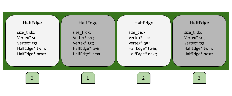
In order to access a halfedge’s neighbor, for example, we would need to access the HalfEdge* twin member and dereference the pointer. Each index in the array also references an entire HalfEdge object. Here is a diagram of the “flattened” version.
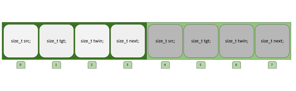
Now we can access any basic information associated with a HalfEdge by indexing into the array (where the start of each halfedge is at an index which is a power of 4) and adding an offset. For example, if we want to get the halfedge twin index from the halfedge at index 1, we would use twin_idx = halfedges[1 * 4] + 2. To add attributes like edge length to a halfedge, we simply make a new array where the indices correspond correctly to halfedges. So, if we wanted to retrieve the length of the twin halfedge we just found, we would use edge_lengths[twin_idx].
Switching to an index-based HEDS gives us the flexibility to easily move our data to and from the GPU memory, and also allows us to add scalar attributes without needing to reallocate or scale an existing array.
Using the GPU with HIP/CUDA
Both HIP and CUDA have very robust C++ bindings that fold into existing projects easily. Since this code was written and tested primarily with an AMD GPU (RDNA3 architecture), we will describe GPU operations with AMD’s HIP runtime. Conveniently, the HIP bindings are essentially CUDA bindings that swap the word cuda with hip, allowing for incredibly easy conversion between the two runtimes. In fact, the HIPIFY tool can convert CUDA code to HIP code without needing the CUDA runtime installed. The HIP compiler can also produce CUDA binaries. More information about the similarity between HIP and CUDA can be found here.
Code executed on the GPU is written as a kernel, which is compiled specifically for the GPU architecture. Kernels are written just the same as normal functions in C++, except they must
- be marked as
__global__,__device__,__host__, etc. to tell the compiler where the code will be run, - return
void, - and only access memory that has been preallocated to their respective device.
Executing a kernel can be done with a hipLaunchKernel(kernel) function or with the triple-chevron syntax kernel<<<blocks, threads_per_block>>>().
Finding Edge Lengths on the GPU
To compute the edge lengths using the GPU, we take the following steps:
- Let n,m be the vertex count and edge count respectively. We allocate a
doublearray of size m on both the host and device to store our length values. - We also allocate a
doublearray of size 3 x n to store each coordinate value of every vertex. Finally, we allocate asize_tarray of size 4 x m to store our halfedges and their reference index values. - We use
hipMemCopy()to copy all values from the host to the device. - Each thread on the GPU is assigned to a halfedge, where it takes the coordinate values for the source and destination vertices and computes the Euclidean distance. The distance value is then written to the edge length array in device memory.
- We call
hipDeviceSynchronize()to make sure every thread finishes their task. After they are all done, we usehipMemCopy()to copy the edge length array on the device back to the host’s memory. - Finally, we can call
hipDeviceReset()to clear the threads and memory of the GPU. We could instead free memory and reset the thread index manually, but use reset for the sake of simplicity.
Finding Vertex Curvature on the GPU
After computing the edge lengths, we have everything we need to compute vertex curvature values with the following steps:
- Reallocate the memory needed for the halfedge array, the edge length array, the vertex-halfedge array, and the vertex curvature array on the host and device.
- Each thread is assigned a vertex. In the kernel, we iterate over each outgoing halfedge with
halfedge.twin.next. We also initialize our total angle as2 * PI_M. - For each outgoing halfedge, we use
halfedge.nextandhalfedge.next.nextto get the other two edges of the triangular face. We can then use the indices of these edges to retrieve the edge length information from the edge length array. - With the edge lengths loaded, we can use the Law of Cosines from before to get the interior angle. The halfedges
halfedgeandhalfedge.twin.twinare lengths a and c, andhalfedge.twinis length b. We also use the HIP internal math functionsaturatef__to clamp the cosine angle. To get the final angle, we callarcos(). - With each angle computed, subtract that value from the total angle. After all adjacent faces have been processed, we can write the final angle total to the vertex curvature array.
Debugging GPU Code
Thankfully, we can use standard printf() statements in the kernel code to help with debugging. For more involved memory debugging, CUDA and HIP have tools to help.
For CUDA, we first want to compile our code with the -g -O0 flags. Then, we can use cuda-gdb [program name], which acts exactly like you would expect when debugging C/C++ using plain gdb.
For HIP, we can compile as usual, then use ltrace -C -e "hip*" [program name] to get a detailed output of our GPU calls. This is especially helpful for when a kernel is not executing, but not throwing a SEGFAULT, either.
Results and Further Directions
Since the current iteration of this project does not scale up to very high resolution meshes, there is not much of a performance improvement over single-threaded performance. Potential bank-conflict issues also slow down the GPU — fixing this would require some sorting (in parallel!) of our data structure before processing.
One improvement that can be made to support high-resolution meshes is sending data to the GPU in “batches” to avoid issues with limited memory. Another is to create partitions of the mesh that can be processed in parallel to avoid bank conflicts. With both of these improvements, we could see much better performance compared to using a single thread.
Finally, slightly reworking the index-based HEDS to be more streamlined would allow us to use the same data structure to compute numerous other geometric values (face area, unit normals, etc.) in parallel. Going even further, we can support geometry-preserving mesh mutations like edge flips in parallel. This opens the door to many different mesh-based algorithms like coarsening, smoothing, or subdivision.