The basics of smooth curvature

For the uninitiated, I find it helpful to have a super quick rundown on the basics of differential curvature before jumping into discrete notions of curvature.

Finding the normal section

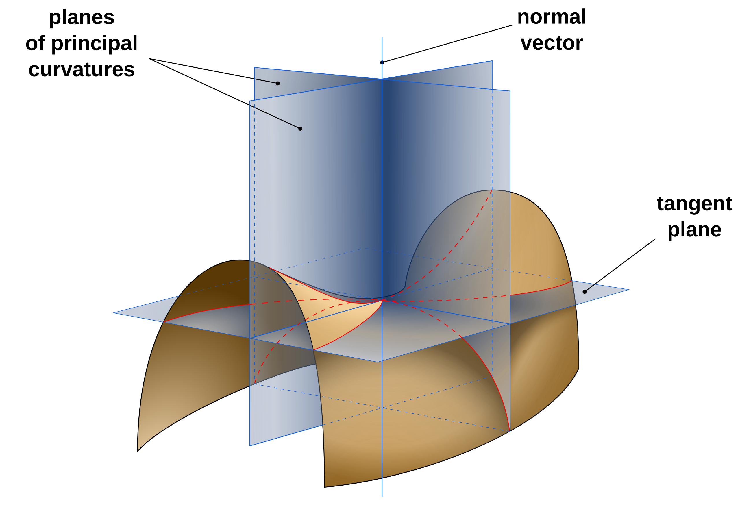
Consider a differentiable surface $X$ in $\mathbb{R}^3$ (in 3-dimensional space) with a defined orientation. At any point $p$ on $X$, we can find a unit normal vector $\vec{n}(p)$ and a unit tangent vector $\vec{t}(p)$. These vectors $\vec{n}(p)$ and $\vec{t}(p)$ define a normal plane, which intersects $X$. That intersection is the normal section, a 2-dimensional curve which we’ll denote as $\mathcal{N}$.

Finding 2D curvature

Now that we have a 2-dimensional curve, we can find the curvature of a particular normal section. Say this curve is defined by $\vec{r}(t)$, with $\vec{r}(t_0) = p$.

On a circle, the curvature of any point on the circle is inverse of the radius ($\kappa = \frac{1}{R}$), so we can define a tangent circle which only intersects the normal section at $p$. Several circles with different radii exist that have this property, however, so how do we know which circle correctly defines the curvature at $p$?

A circle can be defined by any 3 non-collinear points $A$, $B$, and $C$. If we set $A = \vec{r}(t-\epsilon)$, $B = p = \vec{r}(t)$, and $C = \vec{r}(t+\delta)$ with $\epsilon,\delta > 0$, we can define a circle that intersects $\vec{r}(t)$.

In the above demonstration, the green dot represents $B$. As $\epsilon$ and $\delta$ independently approach $0$, the red and blue dots (representing $A$ and $C$ respectively) get closer and closer to $B$. From here, we can write the radius $R$ as a function of $\epsilon$ and $\delta$ and take the limits. The circle with that resulting radius is the osculating circle at $p$.

Recall that $\kappa = \frac{1}{R}$. So, the curvature of $\vec{r}(t)$ at $p$ is

Principal curvatures and Gaussian curvature

At $p$ on the surface $X$, there are a circle’s worth of tangent vectors that can be used to create a normal section $\mathcal{N}$. We label the curvature of a particular normal section $\mathcal{N}$ as $\kappa_\mathcal{N}$. The maximum curvature $\kappa_1$ and minimum curvature $\kappa_2$ correspond to their own normal sections – these are the principal curvatures. We say the Gaussian curvature of $X$ at $p$ is

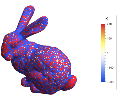
The curvature of a surface at $p$ will look different based on if the Gaussian curvature is positive, negative, or zero. Positive Gaussian curvature means that $p$ is an elliptic point, and that the principal curvatures are the same sign. If Gaussian curvature is negative, then $p$ is a saddle point (or hyperbolic point) with the principal curvatures being different signs. As expected, zero Gaussian curvature means that $p$ is locally flat (developable), like a plane or a cylinder. The best way to demonstrate this is by looking at a torus.

In the above figure, the “outside” of the torus has positive curvature, reflecting that any point in that region has principal curvatures of the same sign. On the “inside” there is negative curvature, once again showing that the principal curvatures at any point in that region have opposite signs.

Discrete Gaussian curvature

Now that we have the basics for finding curvature on a smooth, differentiable surface $X$, let’s try to work in our discrete setting for a surface $Y$.

Trying out differentiable tools

For starters, we can attempt to find curvature of a discrete surface $Y$ using our previous methods. Let $Y$ be a regular hexagonal pyramid with the tip vertex $v$.

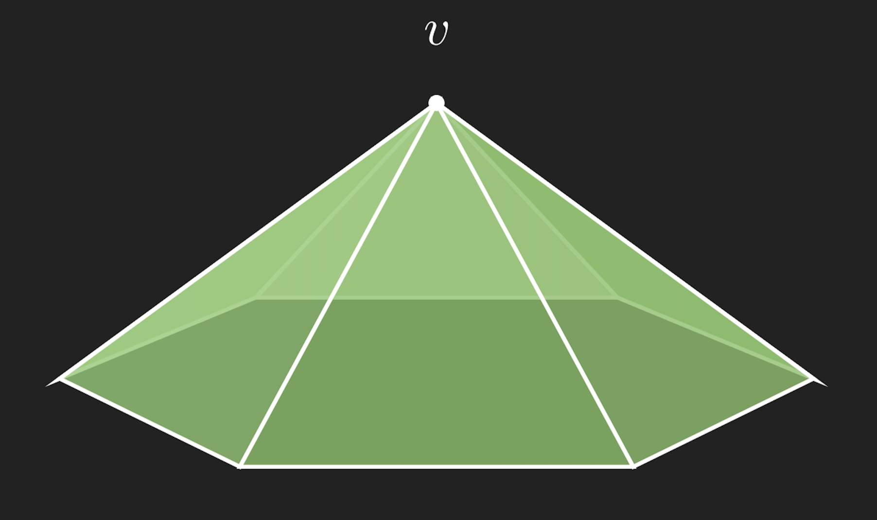
Taking a normal section on any of the faces yields a line, meaning a curvature of $0$. In order to get any useful information, we will want to find curvature at the tip $v$. We end up hitting a roadblock, however – our way of finding differential curvature requires a unit normal vector at $v$, which we don’t know how to find.

While there are several ways that we can define a vertex normal (i.e. a normal vector associated with a vertex), those are outside the scope of this particular post. Lucky for us, we have a simpler solution.

What is angle defect?

Angle defect is the amount the sum of angles fails to add up to $2\pi$, or a complete circle in radians. If you took a piece of paper, laid it flat on a table, and drew a few lines intersecting at the same point, the sum of the angles around that intersection point will add up to $2\pi$ radians. Now if you were to make a paper cone, make a single cut along the side of the cone to the tip, and smushed the cone flat on a surface, you would notice that there’s a “slice” missing. That missing slice is the angular defect.

Take our hexagonal pyramid. If we were to cut out each of the faces and lay them next to each other to make a “pie” shape, we would have a missing angle for our complete circle. Let $\beta_i$ be the $i$th interior angle of a face, and $n$ be the total number of faces on our surface (in this case $n=6$).

The angle defect of $v$ is then

Exactly like differential Gaussian curvature, the sign of the angle defect corresponds to the curvature at the vertex, with positive curvature corresponding to elliptic points and negative curvature corresponding to saddle points. To use the example of the hexagonal pyramid again, the sum of the interior angles is less than $2\pi$ (i.e. the angle defect is positive). This matches our expectation that the shape of $Y$ around $v$ is cone-like.

This simple summation allows computers to calculate curvature on meshes instantly using basic arithmetic, bypassing the complex limits required for smooth surfaces.

Discrete Gauss-Bonnet Theorem and the bigger picture

The Gauss-Bonnet Theorem states that the integral of curvatures on a differentiable surface $M$ is equal to $2\pi$ times the Euler characteristic $\chi$. The Euler characteristic is $\chi = |V| - |E| + |F|$, where $V$ is the set of vertices, $E$ is the set of edges, and $F$ is the set of faces in a mesh. Put together, this is

It turns out that the Discrete Gauss-Bonnet Theorem holds in the same way with angle defect. The sum of angle defects for every vertex on a mesh $Y$ is equal to $2\pi\chi(Y)$:

This connection between the underlying topological characteristics of a surface and its curvature brings substantial implications in mesh manipulation operations. For example, in this paper by Akleman and Chen, it’s shown that establishing minima and maxima for curvature at a vertex can yield more regular triangulations of meshes.