
Analysis of Efficient Matrix Multiplication on the GPU
Matrix multiplication is one of the most commonly used operations in computer science. With the explosion of AI innovations especially, performant matrix multiplication is as critical as ever.
Single-threaded computation is highly inefficient. Multi-threaded computation on the GPU, however, is substantially more performant thanks to its many parallel threads and shared memory caches.
Single-Threaded Matrix Multiplication on the CPU
Computing the product of two matrices is done serially. Assuming that a matrix is stored as a row-major array, single-threaded matrix multiplication is written in C++ as:
void matrix_multiplication_cpu(const float* A, const float* B, float* C, int M, int N, int K) {
  for (auto i = 0; i < M*K; i++) {
    float sum = 0.0f;
    auto row = i / K;
    auto col = i % K;
    for (auto j = 0; j < N; j++) {
      sum += A[row * N + j] * B[j * K + col];
    }
    C[i] = sum;
  }
  return;
}
The multiplication of two matrices, one of dimension $M \times N$ and the other of dimension $N \times K$, has the time complexity $O(MNK)$. We have $(N-1)$ addition operations per entry for $MK$ entries. For the sake of simplicity we will just use the complexity of multiplying two square matrices, which is $\mathcal{O}(N^3)$.
This means that the scaling of this algorithm is terrible. The following benchmark uses a single thread of the Ryzen 5 5600x to compute a series of matrix multiplication operations.
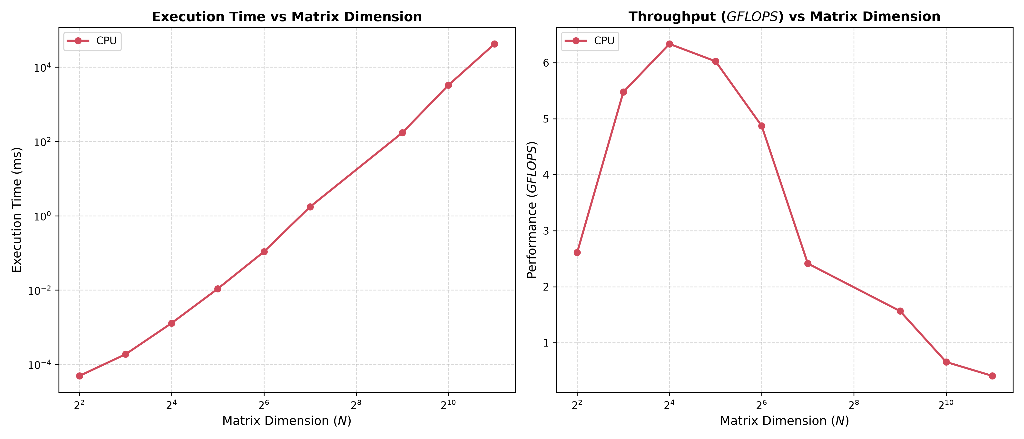
While we can’t do much about the complexity of the algorithm, we can adapt to using a parallel algorithm on multiple threads for better performance at larger matrix sizes. Modern CPUs have multithreading (for example, the R5 5600x has 12 threads), but we can also leverage the thousands of parallel threads on a GPU.
Multi-Threaded Matrix Multiplication on the GPU
CPUs typically excel at complex single tasks with branching paths, working on a single point of data at a time. GPUs are purpose-built for processing lots of data at the same time using a single instruction. This execution model is named “single instruction, multiple threads” (SIMT). Instructions are written as kernels which are compiled and sent to the GPU to run.
GPU architecture organizes its thousands of worker threads into a hierarchy. Threads are grouped together into thread blocks, and all thread blocks are organized into a grid. Each thread block has a shared memory which can be accessed by its threads. All thread blocks can also access a large but relatively slow global memory.
This programming model is supported by the CUDA and HIP languages and APIs. CUDA is maintained by NVIDIA and only compiles to NVIDIA GPUs. HIP, on the other hand, is open-source and maintained by AMD, and also compiles to NVIDIA, AMD, and Intel GPUs. Since I have an AMD GPU, I will be using HIP.
The Very Basics of GPU Memory Management
Because it’s a completely separate device from the CPU, memory on the GPU needs to be explicitly allocated and data needs to be copied over to the allocated memory. This is done via the HIP API:
// create pointers for arrays on the GPU
  float* A_GPU;
  float* B_GPU;
  float* C_GPU;

// allocate the necessary space for the A, B, and C matrices on the GPU
  hipMalloc(&A_GPU, sizeof(float) * M * N);
  hipMalloc(&B_GPU, sizeof(float) * N * K);
  hipMalloc(&C_GPU, sizeof(float) * M * K);

  // copy the values of A, B, and C to the reserved space on the GPU
  hipMemcpy(A_GPU, A, sizeof(float) * M * N, hipMemcpyHostToDevice);
  hipMemcpy(B_GPU, B, sizeof(float) * N * K, hipMemcpyHostToDevice);
  hipMemcpy(C_GPU, C, sizeof(float) * M * K, hipMemcpyHostToDevice);
Kernels can’t directly return values like a C++ function, so the result of A_GPU * B_GPU is stored into C_GPU, then the contents of C_GPU are copied back to C on the CPU. After we’re done using the GPU, we can free memory with hipFree().
Naive Implementation
Someone new to writing parallel programs on the GPU may write a matrix multiplication kernel like so:
__global__ void matrix_multiplication_kernel(const float* A, const float* B, float* C, const int M, const int N, const int K) {
  const unsigned int col = blockIdx.x * blockDim.x + threadIdx.x;
  const unsigned int row = blockIdx.y * blockDim.y + threadIdx.y;

  float sum = 0.0f;

  if (row < M && col < K) {
    for(int i = 0; i < N; i++) {
      sum += A[i + row * N] * B[i * K + col];
    }
    C[row * K + col] = sum;
  }
}
It’s a fairly intuitive implementation. Each thread is assigned an index within its respective thread block, and each thread block is assigned an index within the grid. In this instance, we consider both our block and grids to be 2-dimensional in order to more easily discern which thread maps to which element in the resulting matrix C. We find which column and row the current thread belongs to with:
const unsigned int col = blockIdx.x * blockDim.x + threadIdx.x;
const unsigned int row = blockIdx.y * blockDim.y + threadIdx.y;
After checking that the thread’s index falls within the bounds of C, we compute the dot product of row from A and col from B, then store that result in the corresponding place in C.
`if (row < M && col < K) {
    for(int i = 0; i < N; i++) {
      sum += A[i + row * N] * B[i * K + col];
    }
    C[row * K + col] = sum;
  }
Calculating the efficiency of a parallel program is different from calculating time complexity with a single-threaded algorithm, since the effectiveness of a parallel program is dependent on how well it scales. To do this we use two metrics: work ($T_1$) and span ($T_\infty$).
Work is equal to the time to run the full algorithm on a single processor. This is just the single-threaded time complexity from before, so $T_1 = \mathcal{O}(N^3)$. Span is the runtime of the process given the ideal number of processors. If we have a processor for each entry in C, then $T_\infty = \mathcal{O}(N)$. We can also calculate the parallelism of our GPU algorithm by finding the ratio of work to span:
Putting it simply, this parallel algorithm is much more efficient than the serial one. Theoretically we have reduced the time needed to compute matrix multiplication from being cubically-scaled to linearly-scaled. Of course, no compute has an infinite number of processors, but this result is still informative.
Using the same benchmark as before, we see the substantially more efficient the parallel algorithm is in practice. Note that the dashed line is only the GPU compute time, while the solid line is the compute and memory transfer time.
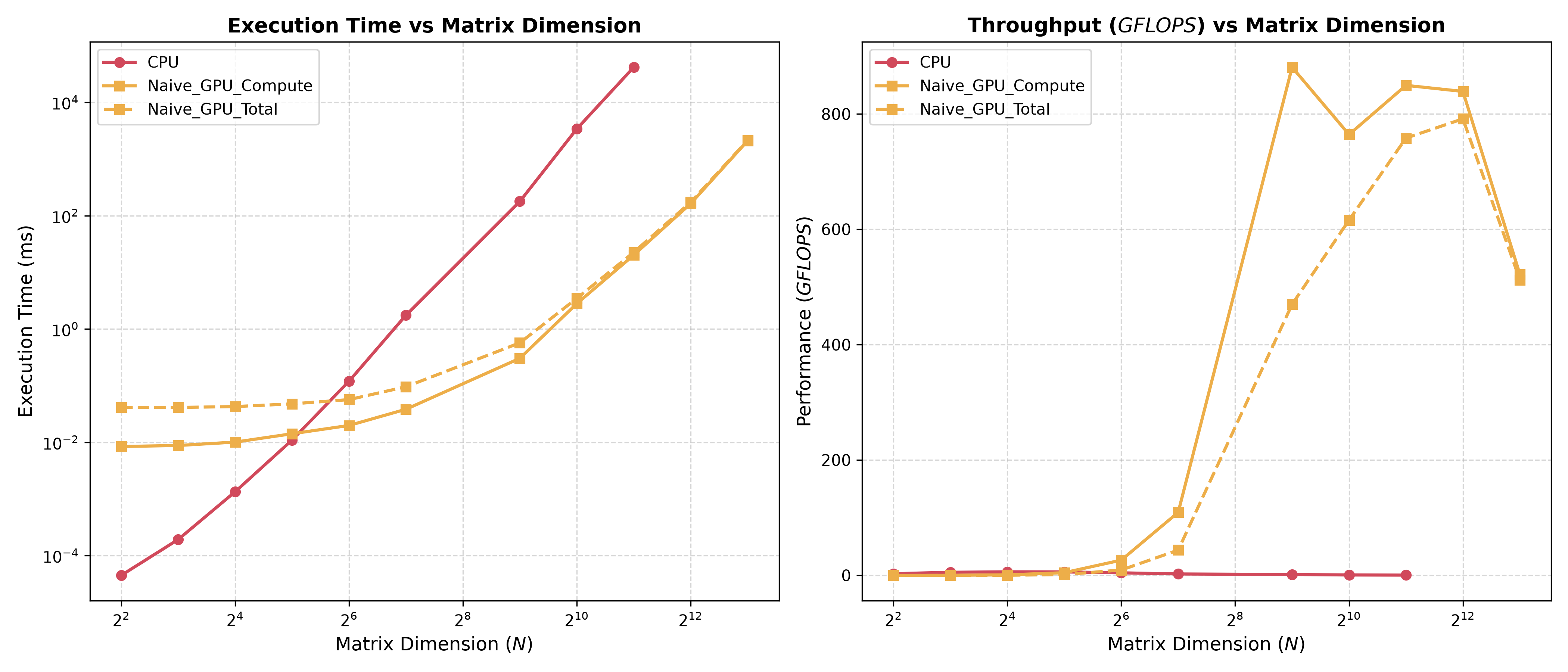
Each thread performs $2N$ arithmetic operations ($N$ addition and $N$ multiplication operations), and $2N$ memory operations ($N$ reads from A and $N$ from B). For $N^2$ threads, that’s $2N^3$ memory and arithmetic operations. Because there are only $2N^2$ elements in A and B, we’re rereading way more than necessary.
We can calculate the arithmetic intensity of the kernel by calculating the ratio of floating point operations (FLOPs) to the number of bytes transferred. As mentioned before, we have $2N$ arithmetic operations per thread. Since we’re working with matrices of floats (which are typically 4 bytes) and reading from both A and B, we have a total of $8N$ bytes transferred from global memory. Thus, our arithmetic intensity becomes:
Right now, our program is memory-bound, meaning the memory operations take up a larger proportion of time compared than arithmetic operations. By Amdahl’s Law, we will see the biggest gains in performance by optimizing the number of global memory accesses and performing more arithmetic operations per byte transferred from global memory.
Optimized Implementation
Every thread block has access to a small but fast shared memory for each of its threads. Shared memory is much faster because it is located on-chip, where the massive global memory is off-chip. By loading data from global memory to shared memory, threads can access the data much faster to perform arithmetic.
The following is the optimized kernel implementation of matrix multiplication on the GPU.
__global__ void matrix_multiplication_kernel(const float* A, const float* B, float* C, const int M, const int N, const int K) {
  const unsigned int row_global = blockIdx.y * BLOCK_DIM + threadIdx.y;
  const unsigned int col_global = blockIdx.x * BLOCK_DIM + threadIdx.x;

  const unsigned int steps = (N + BLOCK_DIM - 1) / BLOCK_DIM;

  float sum = 0.0f;

  __shared__ float shared_A[BLOCK_DIM][BLOCK_DIM];
  __shared__ float shared_B[BLOCK_DIM][BLOCK_DIM];

  for (unsigned int step = 0; step < steps; step++) {
      const unsigned int col_A = step * BLOCK_DIM + threadIdx.x;
      const unsigned int row_B = step * BLOCK_DIM + threadIdx.y;

      if (row_global < M && col_A < N) {
          shared_A[threadIdx.y][threadIdx.x] = A[row_global * N + col_A];
      } else {
          shared_A[threadIdx.y][threadIdx.x] = 0.0f; // Padding
      }

      if (row_B < N && col_global < K) {
          shared_B[threadIdx.y][threadIdx.x] = B[row_B * K + col_global];
      } else {
          shared_B[threadIdx.y][threadIdx.x] = 0.0f; // Padding
      }

      __syncthreads();

      for (unsigned int i = 0; i < BLOCK_DIM; i++) {
          sum += shared_A[threadIdx.y][i] * shared_B[i][threadIdx.x];
      }

      __syncthreads();
  }

  if (row_global < M && col_global < K) {
      C[row_global * K + col_global] = sum;
  }
}
Let’s break this down step by step. First, we set a global variable for the thread block dimensions – in my case, I used BLOCK_DIM = 32 as it matches the wavefront size on the AMD RX 6800XT GPU. We then calculate the global index of each thread with row_global and col_global.
const unsigned int row_global = blockIdx.y * BLOCK_DIM + threadIdx.y;
const unsigned int col_global = blockIdx.x * BLOCK_DIM + threadIdx.x;
We then compute steps, which is the number of times we need to shift our block to load in entire rows and columns. For example, if we have a square matrix of dimension $N\times N$ and our block has dimension $M \times M$, then the number of steps is $\frac{N}{M}$. Of course, $M$ may not divide $N$ — in that case, we round up to the nearest multiple of $M$, padding the final load operation with 0s.
const unsigned int steps = (N + BLOCK_DIM - 1) / BLOCK_DIM;
Now we initialize our shared memory, which is accessible by ever thread in a thread block. We do this using the __shared__ keyword. Note that we create two blocks, one corresponding to A and the other corresponding to B.
__shared__ float shared_A[BLOCK_DIM][BLOCK_DIM];
__shared__ float shared_B[BLOCK_DIM][BLOCK_DIM];
Each step, we have each thread read the value corresponding to its local block index in A and B, then storing those values in their respective shared memory. After we ensure that every thread has loaded its corresponding value from global memory using __syncthreads(), the threads are then free to compute the partial sum for its corresponding dot product. We wait for that to finish again, increment the step (shifting the block to the right in A and down in B), then repeat the process.
for (unsigned int step = 0; step < steps; step++) {
  const unsigned int col_A = step * BLOCK_DIM + threadIdx.x;
  const unsigned int row_B = step * BLOCK_DIM + threadIdx.y;

  if (row_global < M && col_A < N) {
      shared_A[threadIdx.y][threadIdx.x] = A[row_global * N + col_A];
  } else {
      shared_A[threadIdx.y][threadIdx.x] = 0.0f; // Padding
  }

  if (row_B < N && col_global < K) {
      shared_B[threadIdx.y][threadIdx.x] = B[row_B * K + col_global];
  } else {
      shared_B[threadIdx.y][threadIdx.x] = 0.0f; // Padding
  }

  __syncthreads();

  for (unsigned int i = 0; i < BLOCK_DIM; i++) {
      sum += shared_A[threadIdx.y][i] * shared_B[i][threadIdx.x];
  }

  __syncthreads();
}
When every step is complete, the complete sum is written to C in global memory.
if (row_global < M && col_global < K) {
  C[row_global * K + col_global] = sum;
}
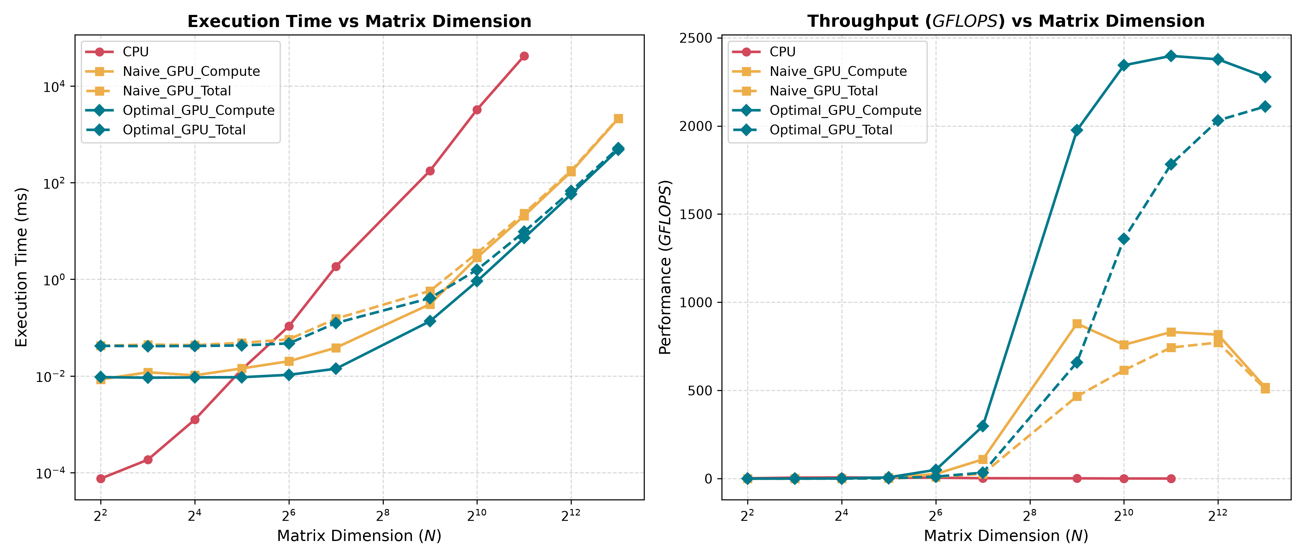
By performing arithmetic from shared memory instead of global memory, we reduce the total number of global memory reads from $\mathcal{O}(N^3)$ to $\mathcal{O}(\frac{N^3}{\text{BLOCK_DIM}})$. We see a substantial improvement in throughput in our benchmark.
Analysis and Conclusion
Developing parallel algorithms for the GPU requires more than simply dividing a workload amongst multiple threads. Multithreading on the CPU usually doesn’t require extensive memory management, whereas carefully managing when memory is transferred to the GPU and which data is loaded into shared memory stores is fundamental to maximizing the hardware’s use. Even operations as fundamental as matrix multiplication see enormous differences in efficiency when tailoring to an architecture’s specifications.
Naive Implementation Analysis
Looking back at the naive implementation from before, we see that there is a noticeable falloff in throughput right after the $N = 2^{12}$ benchmark.
The AMD RX 6800XT used in the benchmark has 128 MiB in its L3/Infinity Cache. At $N = 2^{11} = 2048$, each matrix takes up 16 MiB for a total of 48 MiB. The entire dataset fits inside of the cache as a result.
At $N = 2^{12} = 4096$, however, the dataset balloons to 192 MiB, forcing the GPU to go off-chip to global memory. This introduces significant latency, crippling the number of FLOPs per transferred byte.
Another issue arises from each row of 4096 floats taking up 16 KiB in memory. When traversing columns in matrix B, we step forward 16 KiB in memory, resulting in a guaranteed cache miss due to the set-associative nature of the GPU’s caches.
Optimized Implementation Analysis
Using shared memory is a relatively simple addition that brings an enormous boost to throughput by reducing the number of transactions with global memory. Another benefit of tiling our matrix multiplication is preventing bank conflicts by assigning each row and column a single wavefront.
In my implementation, I set BLOCK_DIM = 32 to match the wavefront size of 32 threads in the RDNA2 architecture. The local data share (LDS) assigned to each block is also split into 32 banks, which allows the scheduler to perform memory transactions in large, singular bursts when the requested addresses are all in their own banks. When the 32 threads request data from shared_B[i][threadIdx.x], each column maps to a thread in the wavefront, which in turn correspond to unique banks, allowing for coalesced global memory reads.
Another neat benefit is that all threads have the same threadIdx.y. When they request shared_A[threadIdx.y][i], each thread is requesting the exact same data, which triggers a hardware-level LDS broadcast that sends the same value to all threads in the wavefront.
Combined with the on-chip benefits of shared memory, avoiding banking conflicts allows our memory transactions to complete in a single cycle. Each tile loaded in from global memory is used BLOCK_DIM times, giving us a global memory footprint of $\mathcal{O}\frac{N^3}{\text{BLOCK_DIM}}$. Our new arithmetic intensity reflects this:
“Embarrassingly” Parallelizable
Matrix multiplication is known to be “embarrassingly parallelizable” — each element in the resulting matrix can be computed completely and totally independently, avoiding the need for inter-thread communication entirely. This is great news for deep learning and graphics programmers, who rely on the GPU being able to efficiently compute millions upon millions of matrix operations. Other use cases require much more complicated programming to make the most of the architecture, however. Effective parallel programming stems from the ability to both analyze the theoretical efficiency of a given parallel algorithm and knowing how to make the most of the hardware available.